Spline - General informations
|
|
Spline - General informations |
Cubic spline
When you create a Spline with TopSolid, it is a non rational cubic Spline (degree 3).
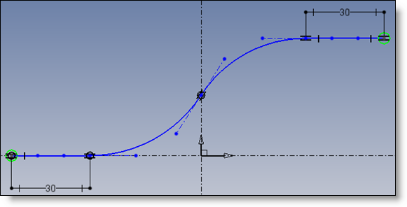
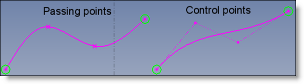
A Spline is a (cubic) polynomial continuous curve segmented as a list of contiguous arcs. The arcs extremities are the interpolation points (also called passing points).
In some cases, it can be useful to define the Spline by attraction points, also called control points.
The cubic BSpline is converted and displayed as a non rational Bezier cubic curve, which is a more geometric representation of the same mathematical object.
A cubic Bezier curve is given by its control points, numbered from 0 to n. The ternaries ones are the interpolation points. The others are the extremities of the left and right tangents.
Each geometric object has a mathematical dimension, or some degree of freedom (Dof).This number is the number of elementary constraint (fixing one dof) one has to set in order the object gets fixed.
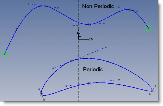
Let NbI be the number of interpolation points (including start and end in the non periodic case), and NbP the number of Bezier points.
|
Bezier cubic spline |
NbP |
Dof |
|
Periodic |
3 * NbI |
6 * NbI |
|
Non periodic |
3 * (NbI – 2) + 4 |
6 * (NbI – 2) + 8 |
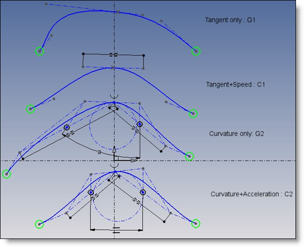
At a Bezier interpolation point, the curve can be more or less smooth. Imagine you are a robot walking on the curve, at a speed which is prescribed by some (good!) master somewhere. This different continuity levels are:
- G0 or connected: no additional constraint to an interpolation point. This is the same left and right! Number of additional constraints, Nbc, is zero.
- G1 or Tangent: the speed direction keeps the same: Nbc = 1
- C1 or Tangent and speed: the speed vector keeps the same (left and right tangents keeps proportional or equal): Nbc = 2
- G2 or Curvature: in addition to C1, the normal acceleration keeps the same direction, which is equivalent to the curvature centers are the same, or the osculation circle is the same left and right: Nbc = 3.
- C2 or Curvature and acceleration: The tangential acceleration is in the same proportion left and right that the normal one:Nbc=4
|
Dof |
G0 |
G1 |
C1 |
G2 |
C2 |
|
Periodic |
6 * NbI |
5 * NbI |
4 * NbI |
3 * NbI |
2 * NbI |
|
Non periodic |
6 * (NbI – 2) + 8 |
5 * (NbI – 2) + 8 |
4 *( NbI – 2) + 8 |
3 * (NbI – 2) + 8 |
2 * (NbI – 2) + 8 |
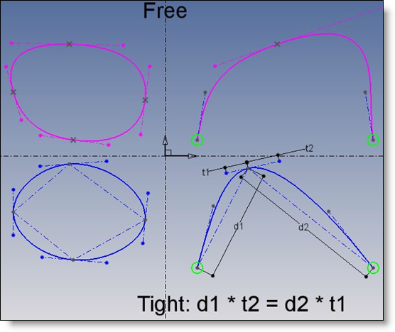
The BSpline (Bezier spline) can be tight or not. Imagine that a spline is a classical cord (no elasticity along his tangent) going throw prescribed points (clamps). And that you pull or push on the cord. If you pull as much as you can, the cord would take a certain shape. This shape will maximize the cord energy, it means minimize the curvature (= 1 / radius) along the curve. Between two points, the cord will be shaped into a line. Between several points, because these are not aligned and that the curvature continuity is preserved, the cord will take a tight shape.
When an interpolation point is fixed and the curve is tight, the curve is losing (3+1) Dof. So we have for the whole curve:
|
Dof |
Tight G2 |
Tight C2 |
|
Periodic |
1 * NbI |
0! |
|
Non periodic |
1 * (NbI – 2) + 4 |
4 |
Important remarks: “Tight case”:
- When periodic, the curve is well constrained.
- When non periodic, one can still fix the start and end tangents!
- The curve is automatically set to C2 when the tight option is used in TopSolid
The curve is tense, and this is not good to design unformed shapes: one cannot tune the curvature. The only way then is to add more and more interpolation points.
When the curve is not tightened, the curve is G2, and the interpolation points are fixed, the curve is losing 3 Dof per interpolation point:
|
Dof |
Free G2 |
Free C2 |
|
Periodic |
2 * NbI |
NbI |
|
Non periodic |
2 * (NbI – 2) + 4 |
NbI + 4 |
Remarks:
When periodic, one keeps only two Dof at each interpolation point. It is not enough to allow moving locally a tangent, the other keeping strictly fixed. So when one drags a tangent end point, the other tangents are moving slightly in length and direction, trying to keep their direction.
To force “more” the other tangents to keep their direction and adjust only in length, one has to use the Alt+Drag mode.
The situation is “worse” in the C2 case. Moving a tangent means moving all the tangents, without being able to keep their directions.
It is a good reason to choose G2 as the standard BSpline case.
When the curve is G2 continuous (this is the standard case), and if the interpolation point and the osculation circle are fixed, the curve is well constrained in the periodic case. Remarkable property.
In the non periodic case, the curve keeps 2 Dof, and one has still to fix the length of the start/end tangents.
In the C2 case, the curve is over constrained and cannot maybe solved.
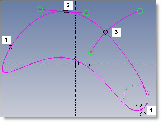
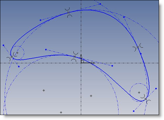
The constraints
|
|
|
1: Point on curve, 2 : Tangent, 3 : Perpendicular, 4 : Curvature |
Cubic ASpline
There is a way to create more sophisticated cubic BSpline, belonging always to category of cubic polynomial curve, but with possibly a rational denominator (Cubic rational Bezier).
The great interest is that it allows representing perfectly the circle, conic, parabola curves as a Bezier like curve controlled by points: it can represent all the usual curves. ASpline means A(ll)Spline!
Arcs types
Each BSpline, which is a list of contiguous polynomial arcs, has a type corresponding to the usual geometric arcs:
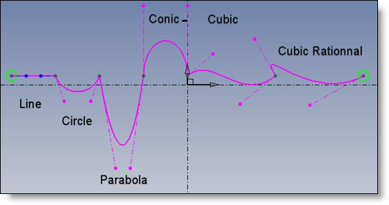
The line is degree 1: no curvature
The circle, parabola, conic arcs are degree 2: they are convex arcs without inflexion points. Curvature has always the same sign.
The cubic and cubic rational are degree 3: the curve can go throw his tangent.
At each vertex intersection of two contiguous arcs, one can define a continuity property:
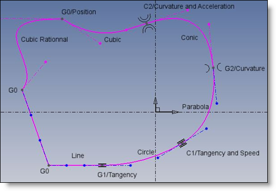
If a point follows the curve with a certain speed and acceleration, following the curve parameterization, it can change of direction, curvature, speed, acceleration at each ASpline vertex.
G0 continuity: everything can change at vertex except the vertex position
G1 continuity: direction is kept
C1 continuity: direction and speed are kept
G2 continuity: direction, speed, curvature are kept
C2 continuity: direction, speed, curvature, acceleration are kept
The curve smoothness increases from G0 to C2.
Examples
|
|
|
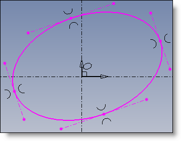
Ellipse |
|
|
|
|
|
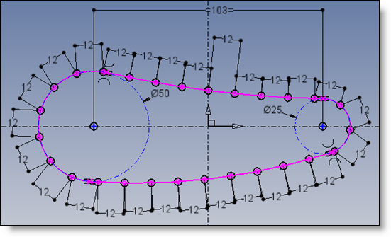
Chain |
|
|
|
|
|
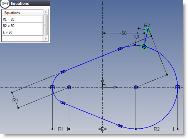
Belt with equations |
|
|
|
|
|
Doucine |